Select the Excel data range
In principle, multiple tasks, and reports with Pivot tables comfortable parallel solve. In our example, we want to determine the number of orders and the turnover of the Region "South". To prepare your data for use in a Pivot table, select the data range first.
- To do this, click in the first cell in your Excel worksheet, press and hold the right mouse button and select the desired area. This area should now be "blue" marks.
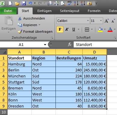
Base data for the pivot table
Creating the Pivot table
- Now click on the "Insert" tab. In the Overview the Symbol for the "Pivot Table"wizard, you click with the left mouse button, appears in the first place.
- Then the wizard, which is available to the further preparation help opens. Due to the selection of your data area in the first section, the options "table or are here already select", and table/field" preset. Excel offers other functions, such as, for example, we take the use an external data source (e.g., Access database or SQL-Server) that at this point, but closer.
- The data area is selected - now you should decide whether your Pivot table should be created in a new or in the existing worksheet. For our example, we use the Option "New worksheet". The Basis of the Pivot table is now created.
Start the Pivot Table wizard
Adjustment of the Pivot table
The next step to your finished Pivot table consists in the fact, adjust the values. This is about the "Pivot Table field list", which you should now be displayed. In the upper area of the field list, you can find the data fields from your selected data range. In the lower part of the columns, you can "report filter", "and row labels" and "values" setting. As mentioned above, we want to determine the number of orders and the turnover of the Region "South". The following adjustment is necessary:
- Drag the Region field in the report filter area. This is necessary to give a filtering to the Region of "the South" to carry out.
- Drag the field "location" in the "row labels".
- The fields for "orders" and "sales", they finally, in the field "values".
Field list
Last finishing touches - The final Pivot table
After you have placed all of the data fields in the Pivot table, you can close the field list. You can at any time out of the table with a click of the right mouse button again to unhide.
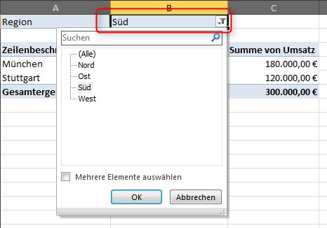
- To fit finally, the Filter of the field "Region" in which you click on the Filter icon, and the value "South" in the select. Thus, the table is created and can be used.
Filter selection
They are Excel-Pro with the new rate in the CHIP Academy
With the course in the CHIP Academy "Excel: Pivot tables in less than an hour" to learn even for beginners, as it is quick and easy, even with a large amount of data to be bypassed.
- You will learn in 40 minutes from our lecturers Daniel Kogan, what Pivot tables are and how to use them wisely.
- You will learn how to draw by using Pivot-tables and Pivot-Charts, findings and insights from your data that would not have developed them otherwise.
- Visit the CHIP Academy and get it for 19,90 euros the extensive Video Workshop in the Online Stream.

CHIP Academy
Microsoft Windows 7 SP1 Microsoft Excel 2010.