All of the format cells based on their values
This Excel-type of rule provides graphical options, for example, numerical values, mosquitoes optically negative. This will provide you with a Overview of your data.
- Select a range in the Excel spreadsheet and click on the Tab "Start".
- Now select "Conditional formatting" and then click "New rule...".
- Select in the new window, type "All cells based on their values format".
Cells color-code with a value above or below
Values that do not fit in a certain area, you can do with Excel easy to find. With this function, the cells do not adhere to a value are marked in colour.
- Select a range in the Excel spreadsheet and click on the Tab "Start".
- You can also go to "Conditional formatting" and then click "New rule...".
- Instead, select "Classic", so you configure that the cells be characterized in a value less than or exceed the colour.
2 - and 3-color scale
You can lend the importance of their values on the basis of a gradient expression of power. They show, for example, on a scale of one to ten, how high is the radiation in an area.
- In the lower area of the window, choose format-style "2-color scale".
- The type you choose for Minimum, "Lowest value" and Maximum "the Highest value".
- If necessary, change the predefined colors and close with "OK". For a 3-color scale, simply set the formatting for the mean.
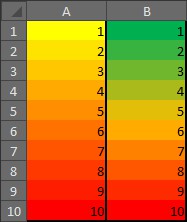
Values with a color scale
Bar
You can use the formatting bar. They represent, for example, your expenditure per month in Excel graphically.
- You simply choose the format, style "data bars".
- The type you choose for the Minimum and Maximum "Automatically".
- You make below the representation of the bars and close with "OK".
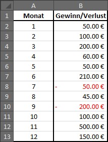
Formatting with beams
Symbol sets
With icon sets you can enter, for example, the signal strength of the network in percentage and with the appropriate symbols, as a graphical means of use.
- Select in the lower pane of the window, the format, the style "icon sets".
- As a symbol type choose the display of the signal.
- In the case of the first Option, "if value:" set this to">". The Rest you can leave it as it. With a click on "OK" the Excel rule.
Values with symbols to represent
Only format cells that contain
This type of format is particularly suited to some special values. For example, all Numbers can be formatted to 0 with the color red.
- Select the range in the table for the formatting to apply and create a new rule with the type "this is the Only format cells that contain".
- You set the following Option: "cell value less than 0"
- Click on the Button "Format..." and select in the new window, as the color red.
- Click twice on "OK" to create the rule
Cells due to formatting content
Numbers displayed as Text
You have pre-defined texts, that will always happen, is also of this type well. This not only saves you time, but also prevents typing errors.
- Select the range in the Excel spreadsheet, the formatting should apply to and create a new rule with the type "this is the Only format cells that contain".
- You set the following Option: "cell value is equal to 1"
- Click on the Button "Format..." and select the Numbers in the new window, the Tab"".
- Links in the side bar, click on "user defined".
- In the text box under the Label "type:", enter the following: "Hello, world!" - the quotation marks are mandatory.
- Click "OK" twice to complete the Whole.
Numbers displayed as Text
Now enter in a cell that is not in your defined area, the number One, appears instead of the Text "Hello world!". Exactly the same, you can specify additional texts for other Numbers.
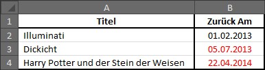
Formula to determine the formatting of cells, use
As the title says, to be formatted, this type of every value for which a certain formula is valid. In this example, all of the Excel are highlighted-data that still lie in the future, red.
- Select the range in the table for the formatting to apply and create a new rule with the type "formula for the determination of the use to format cells."
- Enter the formula =B2>TODAY ().
- Click on the Button "Format..." and select in the new window, as the color red.
- Confirm everything by clicking "OK" twice.
Formatting using a formula
This article shows just a few of the uses of conditional formatting. The function is extremely versatile in use and with a little Routine you can achieve great results. These instructions apply to Excel 2010.