To create 3D Plots in Mathematica
- The Graph that you as a 3D-Plot want to output, must be specified as a discrete Matrix.
- The x-th line is the x-coordinate, the y-th column coordinate of the y. The entry stored in the z-coordinate.
- Mathematica of Cartesian coordinates, with equally spaced entries.
- To create such a Matrix by means of Tables, for example: "mat = Table[Cos[x + y], {x, 1, 2}, {y, 1, 4}];"
- But you can also manually enter values in the Form "mat = {{x1y1, x1y2, x1y3, x1y4}, {x2y1, x2y2, x2y3, x2y4}};".
- "mat" can be plotted by means of the "ListPlot3D[mat]". The values contained in "mat" are the z-coordinates, row and column number for the x - and y-coordinates.
- Using "list density plot[mat]" you can plot the same graph in two space-dimensions. The third Dimension is shown here on the color.

Mathematica 3D Plot example
- To give you a function with two variables, such as "z= Cos[x + y];" for a plane wave. "x", "y" and "z" are the three dimensions of space.
- This function allows you to sample now: "area = Table[Table[z, {x, 0, 3}], {y, 0, 3}];" Here set "{x, 0, 3}" and "{y, 0, 3}" in the range of 0 to 3 in both directions in space.
- "area" looks now so: "{{1, Cos[1] Cos[2] Cos[3]}, {Cos[1] Cos[2] Cos[3] Cos[4]}, {Cos[2] Cos[3] Cos[4], Cos[5]}, {Cos[3] Cos[4], Cos[5], Cos[6]}}"The Matrix notation is shown in the figure.
- By default, Mathematica in steps of One from 0 to 3. Smaller steps you can enter behind the area Definition, to increase, for example, "{x, 0, 3, 0.5}", the spatial accuracy, i.e. increasing x in steps of 0.5.
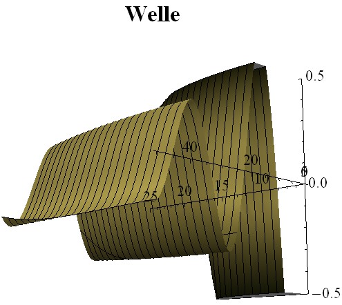
- Using "ListPlot3D[area]" generate graphs of the 3D.
- Two more views of this 3D plot can be found in the photo gallery.

Latest Videos
"ListPlot3D" generates by default a section of the three-dimensional interpolated graph with grid lines, a contoured Box, and the axles.

"ListPlot3D" generates by default a section of the three-dimensional interpolated graph with grid lines, a contoured Box, and the axles.
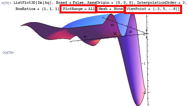
By means of a "Boxed" > "False", you can remove the Box by "AxesOrigin" > "{x,y,z}" the origin of the space axes set.
 "False" you can use the Box remove, by "AxesOrigin" > "{x,y,z}" the origin of the space axes set." />
By means of a "Boxed" > "False", you can remove the Box by "AxesOrigin" > "{x,y,z}" the origin of the space axes set.
The interpolation order can be set by means of "interpolation order" > x". You should not use Box, you need to adjust the aspect ratio using "BoxRatios-> {y,x,z}".
 x" setting. You should not use Box, you need to adjust the aspect ratio using "BoxRatios-> {y,x,z}"." />
The interpolation order can be set by means of "interpolation order" > x". You should not use Box, you need to adjust the aspect ratio using "BoxRatios-> {y,x,z}".
The entire graph display, click on the "plot range" > "All". The grid to remove them by means of "Mesh" > "None" and using the "ViewPoint" > "{x,y,z}" to determine the perspective.
 "All". The grid to remove them by means of "Mesh" > "None" and using the "ViewPoint" > "{x,y,z}" to determine the perspective." />
The entire graph display, click on the "plot range" > "All". The grid to remove them by means of "Mesh" > "None" and using the "ViewPoint" > "{x,y,z}" to determine the perspective.
In order to determine the displayed cutting yourself, type in: "plot range" > "{{xmin,xmax},{ymin,ymax}, {zmin,zmax}}". Make sure that the axes still lie in the plotted area. By means of "Mesh" > "a", a total of signed a grid lines, "Mesh" > "{50, 1}", creates 50 lines in the x and 1 in y-direction.
 "{{xmin,xmax},{ymin,ymax}, {zmin,zmax}}". Make sure that the axes still lie in the plotted area. By means of "Mesh" > "a", a total of signed a grid lines, "Mesh" > "{50, 1}", creates 50 lines in the x and 1 in y-direction." />
In order to determine the displayed cutting yourself, type in: "plot range" > "{{xmin,xmax},{ymin,ymax}, {zmin,zmax}}". Make sure that the axes still lie in the plotted area. By means of "Mesh" > "a", a total of signed a grid lines, "Mesh" > "{50, 1}", creates 50 lines in the x and 1 in y-direction.
Alternatively, there are analytical 3D Plots of the function "SphericalPlots3D", in the function you want to plot, as a function in spherical coordinates given must be.

Alternatively, there are analytical 3D Plots of the function "SphericalPlots3D", in the function you want to plot, as a function in spherical coordinates given must be.
Sometimes, it is the content of a Matrix is not three dimensional, rather than two-dimensional "list density plot[]" or "list of contour plot[]" to spend. In the first variant, the z is encoded axis on the color. In the second variant, the height lines are also marked.

Sometimes, it is the content of a Matrix is not three dimensional, rather than two-dimensional "list density plot[]" or "list of contour plot[]" to spend. In the first variant, the z is encoded axis on the color. In the second variant, the height lines are also marked.


